

[LinkedIn post, Twitter thread, Hacker News discussion]
Table of Contents
Motivation
“Another tutorial on linear regression?!” Someone exclaims. Before I start, I feel the need to clarify what this blog is and is not about. After all, there are probably hundreds if not thousands of tutorials, articles, and online courses on this topic.

But first, let me motivate this topic a little using a quote from text Mathematics for Machine Learning.
Regression is a fundamental problem in machine learning, and regression problems appear in a diverse range of research areas and applications, including time-series analysis (e.g., system identification), control and robotics (e.g., reinforcement learning, forward/inverse model learning), optimization (e.g., line searches, global optimization), and deep learning applications (e.g., computer games, speech-to-text translation, image recognition, automatic video annotation). Regression is also a key ingredient of classification algorithms.
Interestingly, because of its ubiquitous influence in many fields (ML, stats, optimization, control theory, etc.), I found that the notations and solutions to this problem can be inconsistent and sometimes even convoluted1 2 3.
This is where this post comes in. It’s meant to provide a holistic view on different ways to formulate linear regression problem from the perspectives of machine learning, statistics & probability, and optimization. In this post, we’ll introduce linear regression as the most fundamental regression problem. And on top of that, I’ll summarize all the different notations and problem formulations I’ve seen so far.
What it is not about: This post is not a step-by-step tutorial to introduce any specific linear regression concept from stretch.
In this post, I assume that readers don’t have specialized knowledge in ML. If you do, feel free to skip any section that is less relevant for you.
Notation Convention
Notations: There are simply too many notations floating around in machine learning space so in this blog we will stick with using inputs (aka features) denoted by \(x\) or \(X\) (data matrix), output (aka prediction, hypothesis) denoted by \(\hat{y}\), weights (aka parameters) denoted by \(w\) or \(W\), bias (aka error) denoted by \(b\). For more details about different notations please refer to “Miscellaneous: notations” section at the end.
Other notation:
- \(m=\) number of training examples
- \(n=\) number of inputs not including bias
- \(x^{(i)}=\) inputs (features) of \(i^{th}\) training example (i.e. a vector)
- \(x_j^{(i)}=\) value of input (feature) \(j\) in \(i^{th}\) training example (i.e. a scalar)
What’s linear regression?
My first contact with linear regression dates back to 2020, when I took Andrew Ng’s Machine Learning course on Coursera. Simply put, linear regression is an approach to finding a linear equation (model) that takes in one or more inputs and outputs a continuous output variable (target variable).
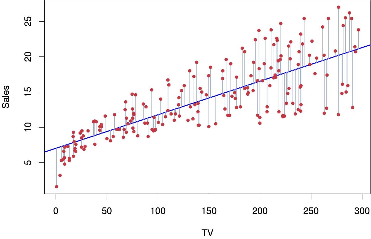
An example could be predicting sales (output variable) based on TV’s advertising budget (input variable). From the graph below, the red dots represent the historic data; the blue line is that linear equation (our model) that we magically found, which outputs the best predictions for both training & testing data (aka “generalize well”).
How do we use the model? Now if I want to predict sales with a TV advertising budget of 200 units using this model, I can trace my finder up from the 200 tick on the x-axis until it meets the blue line (i.e., our model), then trace it to the left until it touches the y-axis. The exercise would give you a prediction about 16–17 units of sales.
Math
We can write out this linear equation (blue line) in a mathematic form:
\[\hat{y} = b + w_1 x_1,\]where \(\hat{y}\) is the output variable, our predicted height, and \(x\) is our input, weight.
A more general format to write it in case we’re dealing with multiple inputs (multi-variate linear regression) is:
\[\hat{y} = b \pmb{x_0} + w_1 \pmb{x_1} + \dots + w_n \pmb{x_n} = XW = \begin{bmatrix} x_0^{(1)} & x_1^{(1)} & ... & x_n^{(1)} \\ \vdots & \vdots & \ddots & \vdots \\ x_0^{(m)} & x_1^{(m)} & ... & x_n^{(m)} \end{bmatrix} \begin{bmatrix} w_0 \\ w_1 \\ \vdots \\ w_n \end{bmatrix},\]where \(\pmb{x_i} \in \mathbb{R}^{m \times 1}\), \(X \in \mathbb{R}^{m \times (n+1)}\) (data matrix), \(W \in \mathbb{R}^{(n+1) \times 1}\), \(\hat{y} \in \mathbb{R}^{m \times 1}\). Note that here we let all \(x_0=1\) for every row in \(X\) to complete the data matrix so that we can include bias as a weight (\(w_0=b\)).
How to fit a LR model?
Each formulation will be discussed in two parts:
- high-level intuition
- some math behind it
I won’t go too deep into the math here as you can find lots of other articles and textbook reference on math. If you’d like, you can totally skip the math part and still understand each formulation pretty well.
Formulation 1: Gradient descent (“the ML way”)
Intuition
Gradient descent is probably the most popular opitimization algorithm right now in the machine learning space, as it’s fundamental to training not only classic ML models but also all deep neural networks that require backpropagation.
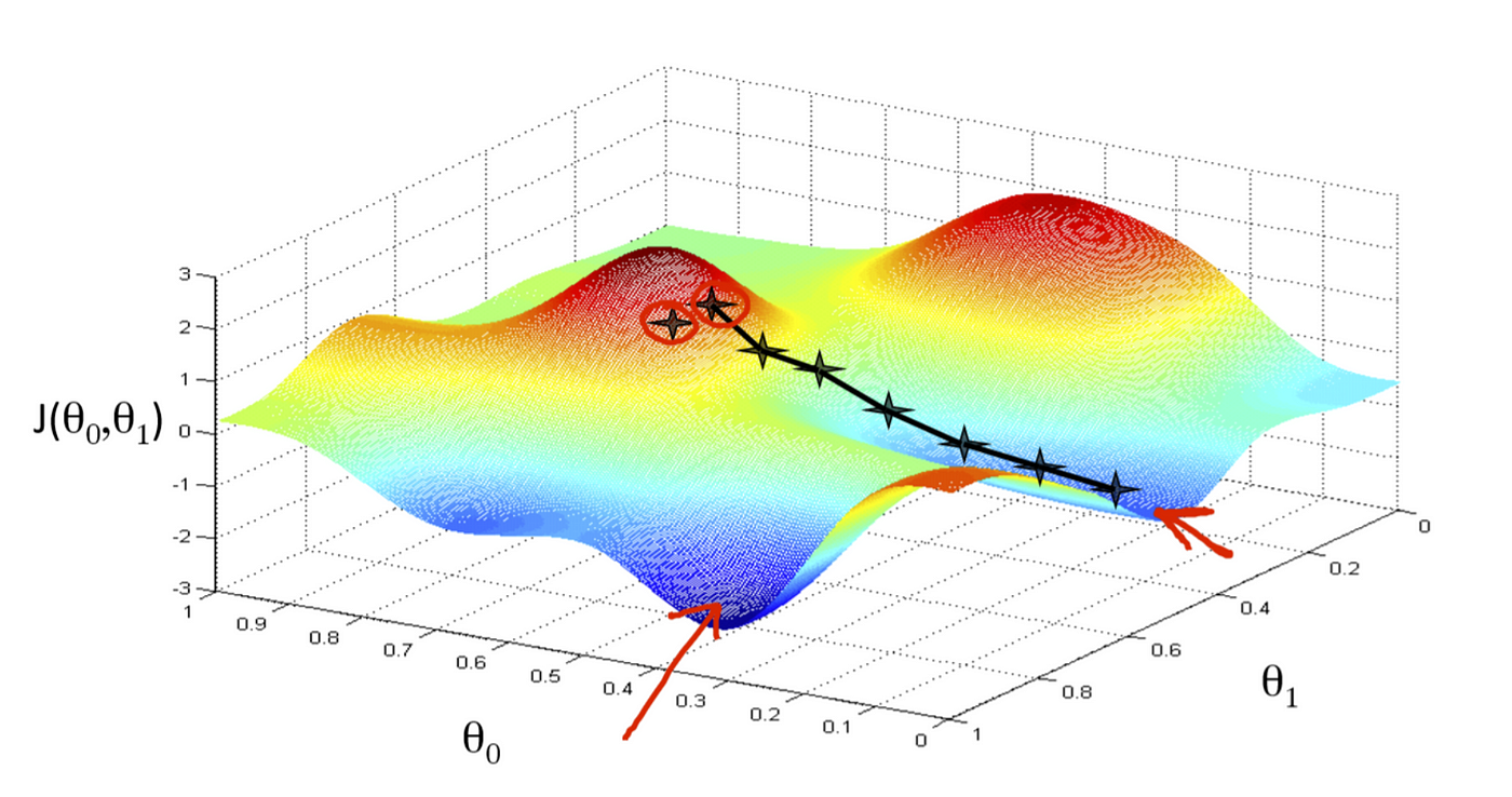
The goal here is to minimize the cost function in high-dimensional space by iteratively taking “small steps” in the direction with a lower cost. One analogy in the 3D world could be descending a mountain from its peak; here, the altitude will be your cost function’s output \(f\). How many weights are you optimizing then? You probably would have guessed—it’s your latitude and longitude (\(w_0\) and \(w_1\) below!). Here’s a visual to help you imagine.
What if we have more than two inputs (features) in our dataset? The math is the same: simply take the partial derivative w.r.t. the weight of each input variable from \(w_0, \dotsb, w_n\) where n is the number of input variables.
A high-level summary of the steps takes in gradient descent is described below:
- Define a cost function \(f(\vec{w})\) (e.g. mean squared error (MSE), mean absolute error (MAE), etc.)
- Minimize \(f(\vec{w})\) using gradient descent technique until the change of \(f\) between iteration \(i\) and \(i+1\) converge within a bound
- Take a step towards the opposite direction of the gradient of cost function
- Adjust \(w\)
- Take another step
- Repeat until convergence
Math
Step 1: Define a MSE cost function \(f(\vec{w})\)
\[f(w) = f(w_0, \dotsb, w_n) = \frac{1}{2m} \sum_i (\hat{y}^{(i)} - y^{(i)})^2 = \frac{1}{2m} || XW - y ||_2\]Step 2: Take the gradient w.r.t each \(w_i\) and update \(w_i\) simultaneously through vectorization
\[w_j := w_j - \alpha \frac{\partial}{\partial w_j} f(w) = w_j - \alpha \frac{1}{m} \sum_{i=1}^m (\hat{y}^{(i)} - y^{(i)})x_j^{(i)}\]Step 3: Compute loss and if \(\Delta f > \text{predefined threshold}\) then repeat step 2 until converge.
Formulation 2: The Normal equation
Intuition
Whenever we approach a mathematical problem, in this case, minimizing our chosen cost function, there are usually two types of solutions: analytical solutions and numerical solutions.
Analytical solutions have a strict logic and return an exact answer; for example, factorizing a matrix using singular value decomposition or other linear algebra methods based on the properties of the matrix.
Unfortunately, there are many problems that do not have an exact solution, such as the travelling salesman problem. A numerical solution makes reasonable guesses and eventually returns a “good enough” solution that meets certain constraints. Gradient descent gives us a numerical solution of weights because it’s nearly impossible to reach the global minimum once you find yourself optimizing a non-convex cost function in a high-dimensional space like neural networks. Machine Learning Mastery gives a more detailed illustration of the differences.
Normal equation is a analytical solution to find exact \(W \in \mathbb{R}^{(n+1)}\) using data matrix \(X \in \mathbb{R}^{m \times (n+1)}\) and ground truth \(y \in \mathbb{R}^{m}\).
Math
Recall previously we’re able to write \(\hat{y}\) in matrix notation:
\[\hat{y} = XW\]Then we can substitute the above expression into the cost function \(f(w)\) to rewrite the sum as matrix notation as well:
\[f(w) = \frac{1}{2m} \sum_i (\hat{y}^{(i)} - y^{(i)})^2 = \frac{1}{2m} || XW - y ||_2\]\(\| \cdot \|_2\) denotes the Euclidean norm of a vector defined as \(\|x\|_2 := \sqrt{x_1^2 + \cdots + x_n^2} = x^Tx\), which is equivalent to the \(\sum\) expression! Now expand the Euclidean norm using matrix transpose identities you will get:
\[f(w) = \frac{1}{2m} (XW - y)^T(XW - y) = ((XW)^T - y^T)(XW - y) \\ f(w) = (XW)^T XW - (XW)^Ty - y^T(XW) + y^Ty\]Note that \(XW\) is a vector, and so is \(y\). So when we multiply one by another, the order does not matter (i.e. \(x^Ty = y^Tx\)). Further simplify the expression into:
\[f(w) = WX^TXW - 2(XW)^Ty + y^Ty\]To find our unknown \(W \in \mathbb{R}^{(n+1)}\), we will derive by \(W\) and compare to zero. Deriving by a vector involves matrix caculus but in the end we just derive by each component of the vector, and then combine the resulting derivatives into a vector again. Eli Bendersky has a wonderfun blog explaining how to derive matrix notation if you’re interested. The result is:
\[\frac{\partial f}{\partial W} = 2X^TXW - 2X^Ty = \vec{0} \\ \Longrightarrow X^TXW = X^Ty\]Now, assuming that the matrix \(X^TX\) is invertible, we can multiply both sides by \((X^TX)^{-1}\) and get:
\[W^{*} = (X^TX)^{-1}X^Ty\]This is the normal equation.
Formulation 3: Minimum likelihood estimation (MLE)
In additional to the first two common ways to look at linear regression, we can take a probablistic approach to formulate the problem and by the end you will see they have very similar steps.
Intuition
Let’s say we get some training examples (i..e our training dataset) and fit a linear regression model (curve fitting) that models these training examples. We assume there’s a function \(f\) that maps inputs \(x \in \mathbb{R}^n\) to corresponding funciton values \(f(x) \in \mathbb{R}\). The ground truths can then be expressed as \(y = f(x) + \epsilon\), where \(\epsilon\) is an i.i.d random variable that describes observation noise, which we have no control of.
The goal is to infer the function \(f\) that generated the training data and generalizes well to new input data. Since we’re dealing parametric models, a parametric estimation method like MLE or MAP can be applied to estimate the best parameters \(W^{*}\) given certain data.
Note: \(\epsilon\) is just the bias \(b\) in formulation 1 and 2 but we choose different notation here to stick with probabilistic convention.
Math
The mathematical expression of the model is given by
\[y = x^TW + \epsilon, \epsilon \sim \mathcal{N}(0, \sigma^2)\]Assuming the noise has a Gaussian underlying distribution and we know its variance for the time being. We obtain the maximum likelihood parameters as
\[W_{MLE} = arg\max_W p(y|X, W) = arg\min_W -\log p(y| X, W)\]To find the optimal parameters, we then minimize the negative log-likelihood
\[-\log p(y | X, W) = -\log \Pi_{i=1}^m p(y^{(i)} | x^{(i)}, W) = - \sum_{i=1}^m \log p(y^{(i)} | x^{(i)}, W) \\ \Longrightarrow \mathcal{L}(W) := \frac{1}{2\sigma^2} \sum_{i=1}^m (x^{(i)}W - y^{(i)})^2 = \frac{1}{2\sigma^2} \sum_{i=1}^m (\hat{y}^{(i)} - y^{(i)})^2 = \frac{1}{2m} || XW - y ||_2\]There you go! So the likelihood function \(\mathcal{L}\) is just as same as the cost function in method 2 with different names. The rest is the same - take derivative of \(\mathcal{L}\) w.r.t the parameters and equalize it to zero and solve for the optimal parameters. And you probably guessed it, the result is just normal equation. However, the amazing part is we started from a very different formulation.
Formulation 4: Maximum a-priori estimation (MAP)
Intuition
MLE and the normal equation are both prone to over-fitting due to its closed-form nature, which means they will fit a curve as perfect as possible given training data. This approach usually won’t generalize to testing data and in reality could be computationally costly to compute the inverse of a matrix.
This is where MAP estimation comes in. We can place a prior distribution \(p(W)\) on the weights. Once a dataset \(X\), \(y\) is available, instead of maximizing the likelihood we seek parameters that maximize the posterior distribution \(p(W \mid X, y)\) to find the optimal parameters.
Math
The posterior over the parameters \(W\), given the training data \(X\), \(y\) is obtained by applying Bayes’ theorem and then followed by a log-transform as
\[\log p(W | X, y) = \log p(y | X, W) + \log p(W) + const,\]where the constant comprises the terms that are independent of \(W\). The MAP estimate will be a “compromise” between the prior (our suggestion for plausible parameter values before observing data) and the data-dependent likelihood.
To find the MAP estimate \(W_{MAP}\), we minimize the negative log-posterior distribution with respect to \(W\), i.e., we solve
\[W_{MAP} \in arg\min_W \{-\log p(y|X, W) - \log p(W)\}\]Formulation 5: Least squares problem
Intuition
Another way to look at a regression problem is to realize that it’s a subset of least squares problem. Imagine that we have a matrix \(A\) of size \(3 \times 2\) (i.e. \(m > n\) more training examples than number of features), then \(Ax = b\) usually does not have a solution. This is called an overdetermined case in least squares problem where we can’t find a perfect solution so instead we seek the least squares solution.
Math
We then try to find set of parameters \(x\) that minimizes the sum of squares of the error
\[\min_{x \in \mathbb{R}^n} ||Ax - b||_2\]the solution of optimal parameters \(x^*\) is
\[x^* = A^{\dagger}b = (A^TA)^{-1}A^Tb\]Again, you will find we arrive at the same answer solved in formulation 2 and 3. This tutorial created by Alex Townsend from MIT does an amazing job at explaining how we can get from least squares problem to normal equation.
Miscellaneous: notations
| Convention used in this blog | Other Notations |
|---|---|
| output variable \(= \hat{y} = \hat{y}(x)\) | prediction, hypothesis (function) \(= h(x) = h_{\theta}(x)\) |
| input variable \(= x/ X\) | predictor, regressor, independent variable, observation / data matrix, feature matrix |
| ground truth \(= y\) | response, label, dependent variable, target variable |
| cost function \(= f(w)\) | loss function, error function, \(J(\theta)\), objective function |
| bias \(= b\) | error \(\epsilon\), observation noise |
| weight \(= w/W\) | parameter \(\theta\), coefficient |
| learning rate \(= \alpha\) | - |
Acknowledgement
Thanks to Ian Webster for reviewing and making this post better.